Minimal introduction to Python

A few years ago I gave a short introduction to Python to some of my former colleagues and this was the result (also on github):

# 1) data basics

# numbers
i = 1234    # integer
f = 1.234   # float

# operators
a = 12 + 5  # = 17
b = 3 * 4   # = 12
c = 6 / 3   # = 2
d = 46 % 5  # = 1 (=> modulo operator)

a += 1      # = 18
a -= 2      # = 16
a *= 2      # = 32
a /= 2      # = 16
a %= 5      # = 1

# text
s = 'string'                
s = s.upper()               # 'STRING'
s = s.lower()               # 'string'
s.startswith('s')           # true
s.endswith('ng')             # true
s = s.replace('str', 'bl')  # 'bling'
l = s.split('i')            # list ['bl', 'ng']
strings = ['s', "t", "r'i'n", 'g"s"tring', "3"]

## add the prefix r for e.g. paths to files to escape the backslash character

testdoc = r'test\test.txt' ## same as : 'test\\test.txt'

# list
l = ['a1']
l.append('b2')
l.append('c3')
l[0] # 'a1'


mixed = ['3', 'abc', 3, 4.56]

d = {} # dictionary (key-value pairs)

d = {'a' : 'blabla',
     'b' : 1,
     3 : 'ablabl',
     4 : 12.3,
     16.9 : 'dif3'}

d['a'] # 'blabla'

# 2) conditions, loops and functions

# indentation is required !!!

if 3 > 2:
    print('3 > 2')
elif 1 == 0:
    print('1 = 0')
else:
    print('else clause')

if 'a' in d:
    print(d['a'])
else:
    print('not found')

for x in range(0, 5):  # from 0 to 5 (0, 1, 2, 3 ,4)
    print(x)

letters = ['a', 'b', 'c']
for letter in letters:
    print(letter)

# list comprehension
upper_letters = [letter.upper() for letter in letters]
print(upper_letters)


d = { 1:'a', 2:'b', 3:'c'}
for key, value in d.iteritems():
    print(str(key), value)
for key in d.keys():
    print('key :', str(key))
for value in d.values():
    print('value :', value)

def special_sum(numberlist):
    total = 0
    for element in numberlist:
        if element < 5:
            continue # go to the next element
        elif total > 100:
            break # stop the loop
        else:
            total += element
    return total

print(special_sum([1,2,2,4,8,50, 60])) # = 118

# 3) using os and shutil

# import modules

import os
import shutil

def setup_test(directory):
    if not os.path.isdir(directory):
        os.mkdir(directory)
    file1 = os.path.join(directory, 'file1_test.dll')
    open(file1, 'a').close() # create empty file and close it
    file2 = os.path.join(directory, 'file2_test.txt')
    open(file2, 'a').close() # 'a' creates a file for appending (doesn't overwrite)
    
setup_test('test')

# looping over files in dir and subdirs and renaming some of them
def list_files(startdir):
    for element in os.listdir(startdir):
        path = os.path.join(startdir, element)
        if os.path.isfile(path):
            print(path)
            root, extension = os.path.splitext(path)
            if extension.lower() == '.dll': # add an extra extension to dll's
                shutil.copyfile(path, path + '.REMOVETHIS')
                # with os.rename you can replace the file
                ## os.rename(path, path + '.REMOVETHIS')
        else:
            list_files(path)

startdir = r'test'
list_files(startdir)

# or you can loop with os.walk

for root, directories, files in os.walk(startdir, topdown=True):
    print 'dir : %s' % root
    if files:
        print('files :')
        for f in files:
            print('\t', os.path.join(root, f))

# 4) reading, parsing and writing files

def create_tab_test(inputpath):
    with open(inputpath, 'w') as inputfile: # 'w' creates a file for (over)writing
        # create some dummy content separated by tabs and with newlines at the end
        lines = ['\t'.join([str(1*i),str(2*i)])+'\n' for i in range(5)]
        # write to the file
        inputfile.writelines(lines)
        
def tab_to_csv(inputpath, outputpath): # only for small files
    lines = []
    with open(inputpath) as inputfile:
        for line in inputfile:
            line = line.replace('\n', '')
            columns = line.split('\t')
            line = ';'.join(columns)
            lines.append(line)
    with open(outputpath, 'w') as outputfile: # overwrites the outputfile if it exists
        outputfile.write('\n'.join(lines))
    
inputpath = r'test\test.txt' ## or 'D:\temp\test.txt'
outputpath = r'test\test.csv'

create_tab_test(inputpath)
tab_to_csv(inputpath, outputpath)

Want to learn more or need some help ?
Contact me at mail@samuelbosch.com or take a look at one of the following resources:
I you want a bigger list of Python and other CS related books to look at then the following free programming books list might be what you're looking for.

-- update --
Some suggestions by Meriam in the comments:

BIOMOD2: invalid term in model formula

While trying out BIOMOD2 for species distribution modeling I encountered the following error when trying to create a random forest (RF) model:

Error in terms.formula(formula, data = data) : 
  invalid term in model formula
Error in predict(model.bm, Data[, expl_var_names, drop = FALSE], on_0_1000 = TRUE) : 
  error in evaluating the argument 'object' in selecting a method for function 'predict': Error: object 'model.bm' not found

After lots of digging in the source code of BIOMOD I discovered what happened and how to fix it.

The line where the error was occurring looked like this:

model.sp <- try(randomForest(formula = makeFormula(resp_name, 
    head(Data), "simple", 0), data = Data[calibLines, 
    ], ntree = Options@RF$ntree, importance = FALSE, 
    norm.votes = TRUE, strata = factor(c(0, 1)), 
    nodesize = Options@RF$nodesize, maxnodes = Options@RF$maxnodes))

As you can see a formula is created from our data. The generated formula looked like this:

654987634 ~ 1 + nitrate_mean + par_mean + sst_mean + sst_range


The number 654987634 is my response variable name that I set when calling BIOMOD_FormatingData which apparently has been added to the Data data.frame as the first column. 


Solution: adding a letter prefix to my response variable name fixed my issue.

Lessons learned:
  1. It's incredibly useful that you can take a look at external source code in an RSession by typing its name, for iternals you add the package name and 3 double dots e.g. biomod2:::.Biomod.Models. Generics functions can be fetched with getMethod e.g. getMethod(biomod2::predict, signature="RF_biomod2_model")
  2. Read the docs very carefully: this is the description for resp.name: response variable name (character). The species name.
  3. An assertion in BIOMOD_FormatingData would have saved me an hour or two. But note that a naive check like is.character(resp.name) wouldn't work in this case, because once the formula is made it isn't a character anymore.
  4. Adding more diagnostic information in your error messages saves people time. If the generated formula would have been printed as well then I would probably have noticed the issue directly.
  5. Libraries make you win time, but you lose some as well.
If you liked this content then don't forget to subscribe on the top left.

Creating a kernel density estimate map in R

In this post I'm going to create a kernel density estimate map in R from a file with latitude/longitude coordinates. WARNING: depending on your application the following gives incorrect results because a non-spherical kernel density estimator is used with spherical data (big thanks too Brian Rowlingson for pointing that out). I didn't find any spherical kernel density estimation implementation in R but if you know any please let me know. While exploring this issue I also wrote a similar implementation as the below code for the generation of a kernel density estimate with the spatial statistics package splancs instead of KernSmooth (splancs_kernel_density.R).

To create this map we'll use the bkde2D function in the KernSmooth package to generate the kernel density estimates and the raster package for outputting a raster file. If you don't have the KernSmooth and raster packages then they can as usually be installed with:

install.packages("KernSmooth")
install.packages("raster")

In order to create the 2D binned kernel density map I first loaded the KernSmooth and raster package.

library("KernSmooth")
library("raster")

Then we read the input file with the coordinates of the points that we want to generate the kernel density estimate off. This input file is an export from the Ocean Biographic Information System (OBIS) and represents distribution records from the seaweed Alaria esculenta.


input <- "Alaria_esculenta.csv"
output <- "Alaria_esculenta_density.asc"

# get the coordinates
records <- read.csv(input)
coordinates <- records[,2:3]

Next we compute the 2D binned kernel density estimate. In order to limit the size of the generated output files I set all values smaller then 0.00001 to 0.

# compute the 2D binned kernel density estimate
est <- bkde2D(coordinates, 
              bandwidth=c(3,3), 
              gridsize=c(4320,2160),
              range.x=list(c(-180,180),c(-90,90)))
est$fhat[est$fhat<0.00001] <- 0 ## ignore very small values

Finally we create a raster file from the output of bkde2D, inspect it visually and export it as an ascii file.

# create raster
est.raster = raster(list(x=est$x1,y=est$x2,z=est$fhat))
projection(est.raster) <- CRS("+init=epsg:4326")
xmin(est.raster) <- -180
xmax(est.raster) <- 180
ymin(est.raster) <- -90
ymax(est.raster) <- 90
# visually inspect the raster output
plot(est.raster)
# write an ascii file
writeRaster(est.raster,output,"ascii")

And the output looks like this. As you can see most records are located near 50°N and 0° which corresponds to the distribution records map generated by OBIS.
The output ascii raster file can be used as an input file for OccurrenceThinner which uses the kernel density estimate grid for filtering out records from densely sampled regions in order to avoid overfitting while building species distribution models (SDM).

Code and data for this post are in my blog github repository.

Azimuthal equidistant projection: An implementation in F#, Python and Julia

Recently I needed to calculate distance from one point to another set of points in order to find the nearest point and its distance to the origin point. I opted to project all points to the azimuthal equidistant projection. The most important property of this projection is that all distances from the center of the projection to all other points represents the true distance (assuming a spheric earth) to all other projected points. To calculate the distance you just have to calculate the euclidean distance and multiply it with the average earth radius (6371000.0 meters).

The formulas for the azimuthal equidistant projection can be found at mathworld.wolfram.com. This formula can then be directly translated into F# like this:

open System
module AzimuthalEquidistantProjection =

    let inline degToRad d = 0.0174532925199433 * d; // (1.0/180.0 * Math.PI) * d

    let project centerlon centerlat lon lat =
        // http://mathworld.wolfram.com/AzimuthalEquidistantProjection.html
        // http://www.radicalcartography.net/?projectionref
        let t:float = degToRad lat
        let l:float = degToRad lon
        let t1 = degToRad centerlat // latitude center of projection
        let l0 = degToRad centerlon // longitude center of projection
        let c = acos ((sin t1) * (sin t) + (cos t1) * (cos t) * (cos (l-l0)))
        let k = c / (sin c)
        let x = k * (cos t) * (sin (l-l0))
        let y = k * ((cos t1) * (sin t) - (sin t1) * (cos t) * (cos (l-l0)))
        (x, y)

I also implemented the azimuthal equidistant projection by using units of measure. I create one set of measures to distinguish between degrees and radians and another one to distinguish between x and y.


open System
module AzimuthalEquidistantProjectionWithMeasures = 
    [<Measure>] type deg // degrees
    [<Measure>] type rad // radians
    [<Measure>] type x
    [<Measure>] type y
    type lon = float<x deg>
    type lat = float<y deg>
    
    let inline degToRad (d:float<'u deg>) = d*0.0174532925199433<rad/deg>
    let cos (d:float<'u rad>) = Math.Cos(float d)
    let sin (d:float<'u rad>) = Math.Sin(float d)
    
    let project (centerlon:lon) (centerlat:lat) (lon:lon) (lat:lat) =
        // http://mathworld.wolfram.com/AzimuthalEquidistantProjection.html
        // http://www.radicalcartography.net/?projectionref
        let t = degToRad lat
        let l = degToRad lon
        let t1 = degToRad centerlat // latitude center of projection
        let l0 = degToRad centerlon // longitude center of projection
        let c = acos ((sin t1) * (sin t) + (cos t1) * (cos t) * (cos (l-l0)))
        let k = c / (sin c)
        let x:float<x> = k * (cos t) * (sin (l-l0)) 
                         |> LanguagePrimitives.FloatWithMeasure
        let y:float<y> = k * ((cos t1) * (sin t) - (sin t1) * (cos t) * (cos (l-l0))) 
                         |> LanguagePrimitives.FloatWithMeasure
        (x, y)

In the past I've used the python OGR bindings and the ESRI Projection Engine for my map projection needs but this time I needed a pure python implementation so I translated the above code and optimized it a bit by precalculating some values that we'll need when we project the points during the initialization of my projection class. A similarly optimized version in F# is on fssnip.net.

from math import cos, sin, acos, radians

class Point(object):
    def __init__(self,x,y):
        self.x = x
        self.y = y       

class AzimuthalEquidistantProjection(object):
    """ 
        http://mathworld.wolfram.com/AzimuthalEquidistantProjection.html
        http://www.radicalcartography.net/?projectionref
    """
    def __init__(self, center):
        self.center = center
        self.t1 = radians(center.y) ## latitude center of projection
        self.l0 = radians(center.x) ## longitude center of projection
        self.cost1 = cos(self.t1)
        self.sint1 = sin(self.t1)
        
    def project(self, point):
        t = radians(point.y)
        l = radians(point.x)
        costcosll0 = cos(t) * cos(l-self.l0)
        sint = sin(t)
        
        c = acos ((self.sint1) * (sint) + (self.cost1) * costcosll0)
        k = c / sin(c)
        x = k * cos(t) * sin(l-self.l0)
        y = k * (self.cost1 * sint - self.sint1 * costcosll0)
        return Point(x, y)

import unittest
class Test_AzimuthalEquidistantProjection(unittest.TestCase):
    def test_project(self):
        p = AzimuthalEquidistantProjection(Point(0.0,0.0))
        r = p.project(Point(1.0,1.0))
        self.assertAlmostEqual(0.01745152022, r.x)
        self.assertAlmostEqual(0.01745417858, r.y)

        p = AzimuthalEquidistantProjection(Point(1.0,2.0))
        r = p.project(Point(3.0,4.0))
        self.assertAlmostEqual(0.03482860733, r.x)
        self.assertAlmostEqual(0.03494898734, r.y)

        p = AzimuthalEquidistantProjection(Point(-10.0001, 80.0001))
        r = p.project(Point(7.935, 63.302))
        self.assertAlmostEqual(0.1405127567, r.x)
        self.assertAlmostEqual(-0.263406547, r.y)

if __name__ == '__main__':
    unittest.main()

I've also implemented the straightforward projection code in Julia. Julia is a promising language built for technical computing. It's still only on version 0.2 but a lot of packages have already been created for the language.


function degToRad(d)
    d*0.0174532925199433
end

function project(centerlon, centerlat, lon, lat)
  t = degToRad(lat)
  l = degToRad(lon)
  t1 = degToRad(centerlat)
  l0 = degToRad(centerlon)
  c = acos(sin(t1) * sin(t) + cos(t1) * cos(t) * cos(l-l0))
  k = c / sin(c)
  x = k * cos(t) * sin(l-l0)
  y = k * (cos(t1) * sin(t) - sin(t1) * cos(t) * cos(l-l0))
  x, y
end

More Python, F#, Julia and geospatial code will be posted here so make sure to subscribe to my e-mail updates on the left. I also occasionally tweet as @gissolved.

What I learned: Part 2 PostgreSQL and PostGIS

In my previous post in the "What I learned" series on Linux commands. Today its time to share some things that I learned while working with PostgreSQL and PostGIS.

Problem: Where are the PostgreSQL logs in ubuntu?

On Ubuntu you can find them here:
cd /var/log/postgresql
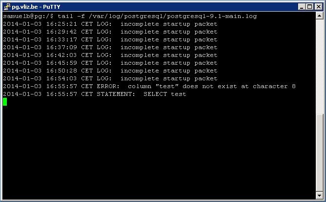
With the tail command you can keep an eye on the logs while it is being written to. On my system the exact command for doing this is:
tail -f /var/log/postgresql/postgresql-9.1-main.log

tail postgresql log

Problem: Copying a subset of a table

I needed to develop some SQL scripts for some very big tables. To be able to quickly test my work I decided to copy the tables to a new schema but with a limited set of records.
CREATE TABLE  AS (SELECT * FROM  LIMIT );
The PostgreSQL documentation contains more information on this topic and some extra samples.

If you also want to copy the original column constraints then its better to create your table with the following two commands:
CREATE TABLE tbl_new (LIKE tbl_org INCLUDING CONSTRAINTS);

INSERT INTO tbl_new 
SELECT col_a, col_b, array[col] aS col_c
FROM tbl_org;

Note that primary and foreign keys and indexes aren't created so if you want them you'll have to create them for your new table.

Problem: Typing the same query over and over again in pgAdmin

Fortunatly you can add macros to pgAdmin with following steps:
  1. Open a query window in pgAdmin
  2. Click Macros -> Manage Macros
  3. Click the key combination that you'd like and type a name and the actual query and hit save.
  4. Repeat for all other macro queries that you'd like
pgAdmin macros screenshot

Some sample macros:
-- inspect the first 100 records of a table. 
-- Select the table and hit the keyboard shortcut you've picked.
SELECT * FROM $SELECTION$ LIMIT 100
-- how many records does a statement return. Also useful for timing queries and subqueries without having to load all the results in your Data Output window.
SELECT COUNT(*) FROM ($SELECTION$) counttable
Some extra information can be found in the official docs.

Problem: Getting the centroid of multiple points in PostGIS

SELECT ST_CENTROID(ST_COLLECT(geom)) FROM points
Note that ST_Collect is many times faster than ST_Union. The difference is that ST_Collect puts the geometries into one multi geometry and ST_Union combines geometries whenever they overlap.

Problem: Creating an array from a query in PostgreSQL

SELECT array(SELECT id FROM table)
Or
SELECT array_agg(id) FROM table

Problem: Repair polygons that are not closed in PostGIS 1.5.4

Solution add the first point at the end of the exterior ring of the polygon when the first point is not the same as the last point. Note that polygons lose their inner rings if there were any. See also: http://lists.osgeo.org/pipermail/postgis-users/2011-December/031615.html
WITH fixed_geom As (
  SELECT gid, ST_Collect(ST_BuildArea(ST_AddPoint(ST_EXTERIORRING(geom), ST_StartPoint(ST_EXTERIORRING(geom)), -1 /* append the point */))) geom
    FROM (SELECT gid,(ST_DUMP(geom)).geom geom FROM qc.global_shorelines) l
   WHERE NOT ST_StartPoint(ST_EXTERIORRING(geom)) = ST_EndPoint(ST_EXTERIORRING(geom))
   GROUP BY gid
)
UPDATE qc.global_shorelines gs SET geom = f.geom
  FROM fixed_geom f
 WHERE gs.gid  = f.gid

Problem : Executing a SQL script within psql

If you want to execute a SQL script within psql then start psql and type:
\i "path .. to .. file"

Problem: Cancelling a command with psql 

To cancel a command hit Ctrl+c and to quit Ctrl+d. An alternative for quitting is typing \q.

Problem: Writing output of psql to a file

If you want to redirect psql output to a file instead of to the prompt then type:
\o filename.here
Type \o again to restore to the standard output.

Problem: Get execution time from query in psql

\timing

Problem: Listing the open connections and active sql queries

SELECT datname,usename,procpid,client_addr,waiting,query_start,current_query FROM pg_stat_activity;

Problem: killing all open connections to a database

SELECT pg_terminate_backend(pg_stat_activity.procpid)
FROM pg_stat_activity
WHERE pg_stat_activity.datname = 'YOUR_DATABASE_NAME'
  AND procpid <> pg_backend_pid()

Problem: Copying data from one server to another with psql

\c dbname username source_db_server
COPY (SELECT * FROM your_table WHERE some_filter) TO '/data/table_copy';
\c dbname username destination_db_server
COPY '/data/table_copy' TO your_table

Problem: On the fly compression of the copy output

To solve this problem in PostgreSQL 9.3 an option was added to the COPY command to directly pipe the output through an external program.
This can be used to pipe the copy output to gzip in the following way:
COPY test TO PROGRAM 'gzip > /data/test.gz';
To achieve the same behavior on older systems you can copy to STDOUT with psql and then pipe this to gzip.
psql -c "COPY test TO STDOUT WITH CSV" | gzip > /data/test.gz

Problem: Tired of typing your password

After filling in my password for the n-th time while using tools like pg_dump and pg_restore I searched for a solution:
export PGPASSWORD=

Conclusions

I hope some of the tips on PostgreSQL and PostGIS might come in handy some day. If you want to learn more on PostgreSQL I would suggest you to check the excellent documentation. For all things related to performance there is the excellent book: PostgreSQL 9.0 High Performance.
The best book on PostGIS is definitely PostGIS in Action. The second edition is coming out in may 28, 2014.

Related Posts

Loading and querying spatial data with PostGIS
What I learned: tmux, top, ls and pscp